Winkler AM, Greve DN, Bjuland KJ, Nichols TE, Sabuncu MR, Håberg AK, Skranes J, Rimol LM
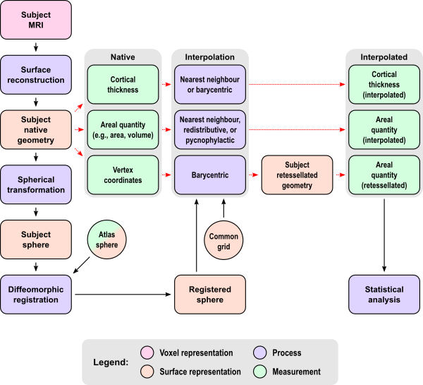
The figure below shows an overview of the steps for the analysis of surface area and the relationship between different methods. The magnetic resonance images (MRI) for each subject are used to reconstruct a pair of surfaces (pial and white) representing the cortex, which initially are in the native space of each subject, using an individual geometry. From this pair of surfaces, cortical thickness, area and volume can be measured. Finally, the coordinates of the vertices can be stored for subsequent use. The subject native surfaces are homeomorphically transformed to a sphere, registered to a spherical atlas, and used for the interpolation (resampling), which for thickness can be either nearest neighbour or barycentric, for area can be nearest neighbour, redistributive or pycnophylactic, and for the vertex coordinates can be barycentric. In the latter, the interpolation of coordinates allows the construction of a new retessellated surface in subject space, from which area can alternatively be measured. The interpolated quantities are then ready to undergo statistical analyses. See references in the main text.

The dashed arrows (in red) indicate separate, mutually exclusive branches; the continuous arrows (in black) apply to all cases, including all within the larger gray boxes.
A detailed comparison of the four interpolation methods, assessed via correlation (scatter) plots, Bland–Altman plots, spatial maps for group differences, group correlations, averages, and standard deviations both at the group level (considering all subjects) and at the subject level for 12 subjects selected by chance. The comparisons use three different resolutions for the target for the interpolation (ic3, ic5 and ic7) and two registration methods (FS: FreeSurfer method; SD: Spherical Demons). See the main text for references.
| ic3 | ic5 | ic7 | ||||
|---|---|---|---|---|---|---|
| Scatter plots | FS | SD | FS | SD | FS | SD |
| White surface maps | FS | SD | FS | SD | FS | SD |
| Pial surface maps | FS | SD | FS | SD | FS | SD |
| Inflated surface maps | FS | SD | FS | SD | FS | SD |
| Global area | — | — | — | — | FS | — |
| FWHM = 0 | FWHM = 10 | |||||||||||
|---|---|---|---|---|---|---|---|---|---|---|---|---|
| ic3 | ic5 | ic7 | ic3 | ic5 | ic7 | |||||||
| Bland–Altman plots | FS | SD | FS | SD | FS | SD | FS | SD | FS | SD | FS | SD |
| Correlation plots | FS | SD | FS | SD | FS | SD | FS | SD | FS | SD | FS | SD |
| White surface maps | FS | SD | FS | SD | FS | SD | FS | SD | FS | SD | FS | SD |
| Pial surface maps | FS | SD | FS | SD | FS | SD | FS | SD | FS | SD | FS | SD |
| Inflated surface maps | FS | SD | FS | SD | FS | SD | FS | SD | FS | SD | FS | SD |
| Total area tables | FS | SD | FS | SD | FS | SD | — | — | — | — | — | — |
| Spatial correlation tables | FS | SD | FS | SD | FS | SD | FS | SD | FS | SD | FS | SD |
A similar comparison for two volume measurements: "volume" is the conventional volume, produced through the multiplication of thickness by area; "newvol" is the proposed analytical cortical volume. For these analyses, nearest neighbour interpolation was used, with the FreeSurfer registration.
| ic3 | ic5 | ic7 | |
|---|---|---|---|
| Scatter plots | FS | FS | FS |
| White surface maps | FS | FS | FS |
| Pial surface maps | FS | FS | FS |
| Inflated surface maps | FS | FS | FS |
| FWHM = 0 | FWHM = 10 | |||||
|---|---|---|---|---|---|---|
| ic3 | ic5 | ic7 | ic3 | ic5 | ic7 | |
| Bland–Altman plots | FS | FS | FS | FS | FS | FS |
| Correlation plots | FS | FS | FS | FS | FS | FS |
| White surface maps | FS | FS | FS | FS | FS | FS |
| Pial surface maps | FS | FS | FS | FS | FS | FS |
| Inflated surface maps | FS | FS | FS | FS | FS | FS |
| Total area tables | FS | FS | FS | — | — | — |
| Spatial correlation tables | FS | FS | FS | FS | FS | FS |
Scatter plots showing the relationship between cortical thickness, area, and volume, as well as Bland–Altman plots comparing the two methods to assess volume, are available here.
For the analysis of variability of the cortical indices, nearest neighbour interpolation was used, with FS registration and the ic7 resolution.
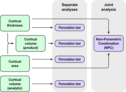
For the statistical analysis, nearest neighbour interpolation was used, with FS registration and the ic7 resolution. Thickness, area and volume (both methods, i.e., multiplicative and analytic) can be analysed separately via permutation tests, or NPC can be used to jointly investigate changes in thickness and area, replacing what otherwise would be the role of volume; the latter is influenced mostly by area only, with a poor association with cortical thickness.

The results are for two contrasts of parameter estimates:
For each case, two models were run: (i) either without any global variable as nuisance and (ii) with global cortical thickness and global surface area; the latter are indicated in the tables under the caption "nuis". The NPC results are either using concordant signs, or with the thickness with the signs reversed (indicated by the word "opposite"). Results for a conjunction (IUT) are also shown.
In the table, "fwep" indicates that the p-values have been corrected for familywise error rate across vertices (both hemispheres); "cfwep" indicates that these p-values have been further corrected across both contrasts (positive and negative, i.e., C1 and C2).
| White | Pial | Inflated | ||
|---|---|---|---|---|
| FWHM = 10 mm |
cfwep | open | open | open |
| fwep | open | open | open | |
| FWHM = 30 mm |
cfwep | open | open | open |
| fwep | open | open | open | |