Composite Linear-nonlinear Regression with Gene Expression ProgrammingBy Yanchao Liu
Optimization-based machine learning models, including Support Vector Machine (SVM), Linear/Polynomial/Logistic Regressions and their regularized variants (such as LASSO, LARS, Elastic Net and Ridge), all assume a known functional form between the input and output variables. Based on this assumption, optimization problems are solved to find the best-fit coefficients for the functions. For example, logistic regression fits a logit-linear function which maximizes the conditional likelihood of the training data, and SVM maximizes the margin between points closest to a separating hyperplane. In optimization terms, such models are convex problems which are in general efficient to solve, and scale increasingly well to large data sets thanks to advancements in optimization algorithms (e.g., stochastic coordinate decent, ADMM) as well as high-performance computing (HPC) infrastructure. However, machine learning literally means letting machines to "learn". To effective and creative learning, too much assumption (aka restriction) is a hinder rather than a helper. In the regression context, it boils down to the question: can we NOT specify a functional form, but let the computer figure one out and fit the coefficients? This question is particularly meaningful if considered with the fact that when we do specify a function, it is mostly for mathematical convenience (e.g., continuity, convexity, closedness, etc.) rather than for any belief that the variables intrinsically follow the function. In this sense, conventional regression analysis EXPLAINS the data variation using predefined function forms, instead of MINING the data for unknown, and possibly truer, relationships in a broader functional space. Consider a pedagogical example: from the data below, how can we, human and computer working together, uncover the true underlying function "y = 1.23*a^(0.5*sin(b)) + a*c + 5.5"?
              y         a          b         c
              -------------------------------------
              28.8932   27.8498    2.6500    0.7431
              27.3979   54.6882    5.7537    0.3922
              68.3986   95.7507    4.9776    0.6555
              22.7096   96.4889    6.0287    0.1712
              17.0200   15.7613    4.1201    0.7060
              10.6360   97.0593    0.2244    0.0318
              32.1991   95.7167    5.3352    0.2769
              8.3037    48.5376    5.8685    0.0462
              13.4439   80.0280    4.2646    0.0971
              17.5108   14.1886    4.7610    0.8235
              ...       ...        ...       ...
The above example is probably unimpressive for practical statisticians/data scientists, because a "true model" rarely exists, especially in social science applications where big data blossom. For most of us, a simple model that sufficiently explains would be good enough (reminiscent of George Box's famous remark: All models are wrong, some are useful.). Nevertheless, the same question persists in a different form: how do we create/define variables (or features) from data to maximize their explanatory/predictive power in a simple, say, linear, model? In predictive modeling, variable creation is where machine learning is least used. Because there are countless ways, angles and granularities in which high-demensional data1 can be viewed and tabulated, human judgement is usually the first pass to trim down the possibilities. Decisions can be tough to make and made ones are subjective at best. For instance, in predicting customers' likelihood of purchase, we know that recent web browse/search activity on the target title is an important factor; one question is how to discretize the time axis and quantify the level of recency. Should we track activities in the past 2 days, 10 days, or 30 days? There are numerous places for the cutpoint, and what's best (in terms of coefficient of determination, for example) is hardly known, a priori and even a posteriori. In practice, we probably end up creating a variable for each plausible scheme. As a result, there can be tens to thousands of variables after the initial round of variable creation, depending on the problem complexity as well as the modeler's level of comfort. Creating an explanatory variable is analogous to projecting raw data points to a subspace relevant to the problem at hand. The projection involves math (set) operations such as max, min, union, sum, etc. To create a variable counting days past since a customer's last transaction, for example, we first slice out all transactions pertinent to the customer, then take the maximum date among these transactions, and subtract it from the current date to obtain the days elaspsed. In this process, the functions "max" and "-" are applied. Math functions are also commonly used in deriving new variables from existing ones (so-called transformation). Here are some examples:
Given an initial set of variables, applying math functions on them is at the core of creating something more powerful. The above listed transformations are simple and intuitive. How about those numerous other more complicated, unintuitive and completely beyond reasoning ways of functional application, such as a^(0.5*sin(b))? Is there a way to systematically unlock those potentials with minimal confinement? We provide a GEP-based software tool to automate this exciting task. Downloads
UsageTo display the usage, run the program without any argument:$ ./geptool Output: Usage: ./geptool [options] infile [outfile] Gene Expression Programming for Regression -v# Read first # available input vars from infile (default: 26) -o* Set of 1-operand function symbols (default: ACDELQRS) -O* Set of 2-operand function symbols (default: +*-/^) -i# Maximum iterations (default: 10000) -n# Maximum rows to read from input file (default: 10000) -h# Head length of a gene (default: 5) -c# Percentage of the population to keep for next iter (default: 0.100) -e# R-square target (0~0.999)(default: 0.950) -m# Mutation rate (0~1) (default: 0.500) -x# Crossover rate (0~1) (default: 0.400) -X# Inversion rate (0~1) (default: 0.100) -p# Population size (default: 100) -b# Number of GEP passes (default: 3) -q# Verbose level (0~2)(default: 1) -t# Number of threads (0~10)(default: 4) -s# Random seed (default: 8888) -! Print additional help information infile File to read data from [required] outfile File to write solution to [optional]To run on a data file (input1.txt) with all options at default level: $ ./geptool input1.txt Input data file should follow this convention: each line is an example (aka. observation, record), columns must be seperated by any of: space, tab, comma or semicolon. Except for an optional header line (first line), all other lines must contain only numeric values. The first column is automatically treated as the target (aka. dependent, output, response) variable, all subsequent columns are feature (aka. independent, input, regressor) variables, internally labeled as a, b, c, .... Examples: input1.txt input2.txt The output (stdout) of the above command is listed below, followed by a more detailed annotation. Output:Gene Expression Programming for Regression Reading 2 input variables per row. 100 rows are read from input1.txt. Elapsed 0.0 seconds. The first 10 rows (with the header line): y(target) a(a) b(b) 11.450000 45.556000 0.190000 48.055000 59.920000 0.891000 37.353000 46.345000 0.875000 14.541000 69.441000 0.302000 16.364000 67.475000 0.424000 19.790000 84.676000 0.469000 12.161000 59.644000 0.228000 79.178000 79.676000 0.962000 13.560000 57.337000 0.329000 10.283000 41.775000 0.082000 R-square of each input variable: a: 0.094 b: 0.725 Using 4 of the 80 processors on this machine. # terminals = 2, # functions = 13, Head Length = 5 1-operand functions: ACDELQRS, 2-operand functions: +*-/^ Crossover = 0.400, Inversion = 0.100, Mutation = 0.500, Cutoff = 0.100 Max iter = 10000, Popsize = 200, R-square target = 0.950 Iter 0: (sqrt((a^b))/cos((b/a))) R-square = 0.944 Iter 2: (((a^b)*exp(b))-exp(b)) R-square = 0.983 Converged at iteration 2, R-square = 0.983 (((a^b)*exp(b))-exp(b)) CPU time 0.0 seconds. Wall time 0.0 seconds. These plots illustrate the data as well as the GEP solution: 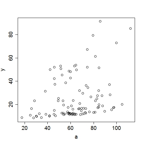
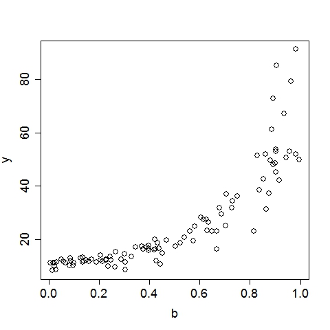
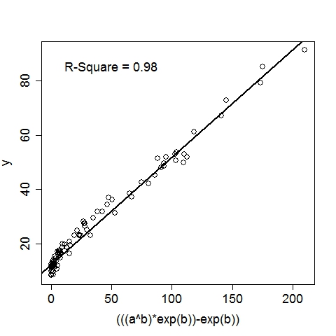
Annotation:The program recognized that there are 3 columns in input1.txt. The first column is by convention the target variable, hence it read 2 input variables per row. By default, the program reads the first 10000 available rows from the input file, this can be changed by setting the option, e.g., -n20, to read the first 20 rows. Since there are only 100 rows in input1.txt, it reads in all 100 rows. The program then displays the first 10 rows (regardless of the total number of rows read) for a visual sanity check. At this point, the data is successfully loaded to memory. Before looking for complicated functions, the program first checks the linear fit between the target variable and each of the input variables. The coefficient of determination, i.e., R-square, is reported. If the best single-variable R-square is already greater than the R-square target (by default 0.95, can be set by option -e0.99 to 0.99, for example), there is no need to look further and the program will terminate. This is apparently not the case here, so the program continues. The program is ready to do some serious work now. The next four lines list the algorithmic parameters to be used in this run (all of which can be set with command-line options). For this particular case with default options:
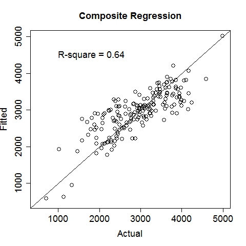
Composite RegressionThe power (and the main point of innovation) of this tool resides in the composition of functions via multiple passes of the GEP run. After each run, the best fit function (in the form of b0 + b1*F(x), where F is a nonlinear function of the input vector x) is used to generate a new variable, which is automatically fed into the next run along with existing variables. Multiple passes create a chain (or a composite) of functions, which advances the fitness performance much faster than the conventional GEP algorithm. Furthermore, it naturally incorporates meaningful numeric constants (i.e., b0's and b1's) in the solution process. Note that each pass will take away two degrees of freedom (DF), hence too many passes may cause overfitting when sample size is small. The maximum number of passes can be specified via the option, e.g., -b10, for 10 passes. (In the current implementation, this parameter is limited to (26 - #vars). For instance, if the data contain 16 input variables, at most 10 passes will be allowed.) The overall execution terminates upon any of the three conditions: (1) when the R-square target is met, (2) when the maximum number of passes is reached, or (3) when the best-found R-square in the current pass is no greater than that of the previous pass. Upon termination, the best-found composite function is saved to the outfile (if specified) in binary format.The following command runs 10 passes on the input data train_elecdemand.txt, at 30000 iterations per pass, across 20 threads and with an R-square target of 99%. The solution is saved in the file sol_elecdemand. All other options are at default levels. $ ./geptool train_elecdemand.txt sol_elecdemand -b10 -e0.99 -i30000 -t20 The run log (stdout) is saved to runlog.txt (by appending "> runlog.txt 2>&1 &" at the end of the above command; otherwise, stdout/stderr is displayed on the screen by default). The process of applying the solution to make predictions on new (or test) data is called scoring, which is facilitated by the program gepscore. (Download: gepscore for Linux, gepscore.exe for Windows.) Its canonical usage is: $ ./gepscore Usage: ./gepscore keyfile indata outdata Apply the key to the indata to generate outdataFor example, the following command generates predictions for the validation dataset valid_elecdemand.txt: $ ./gepscore sol_elecdemand valid_elecdemand.txt output_valid.txt Is the first column of data the true response [y/n]? y Reading 4 input variables per row. 168 rows are read from valid_elecdemand.txt. Predictions are written to output_valid.txt. R-square = 0.931If the indata is a validation set for which the true target (response) is known, the target must occupy the first column and input variables should be arranged in subsequent columns. If the indata is a test set for which the true target is unknown or hidden, the input variables should start from the first column. In either case, the order of the input columns must remain the same as that of the training set (in this case, train_elecdemand.txt) from which the keyfile (in this case, sol_elecdemand) is generated. Whether indata contains the true response in the first column is indicated by a [y/n] answer to the program's question. The predictions are written to the outdata (in this case, output_valid.txt). ExamplesElectric Load ForecastingElectric load is fitted as a linear function of a nonlinear function of time and temperature. 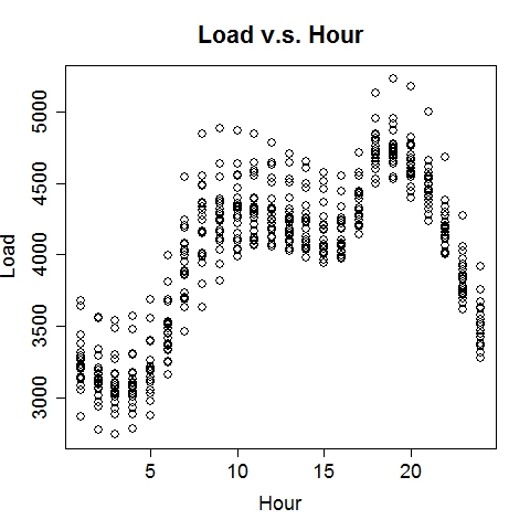
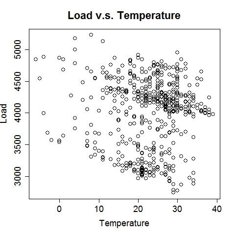
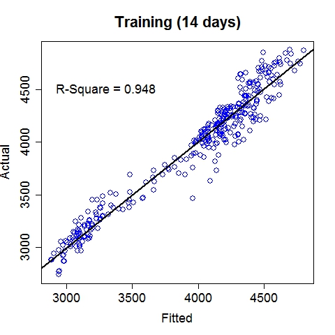
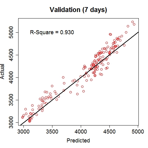
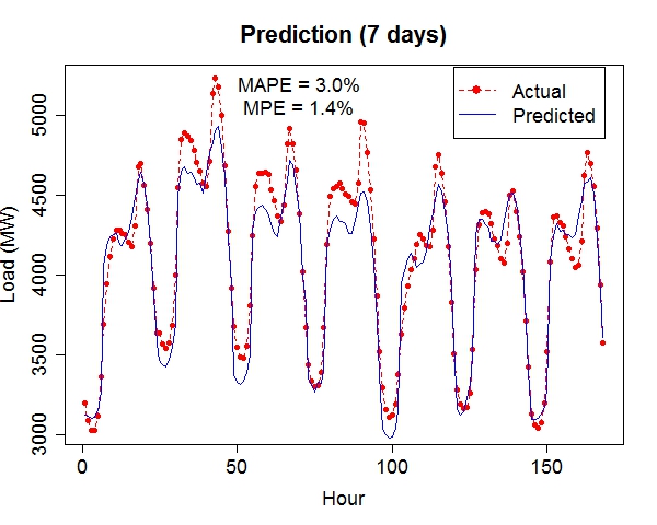
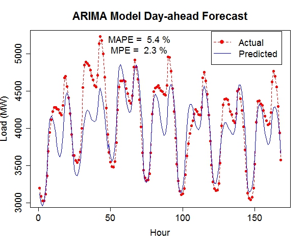
The 7-day forecast (middle figure above) is more accurate than day-ahead forecasts (right figure above) made by a time series model (R code: plot_it.R), in terms of mean absolute percent error (MAPE) and mean percent error (MPE). Low Birth Weight
Data file: LowBirthWeight.txt 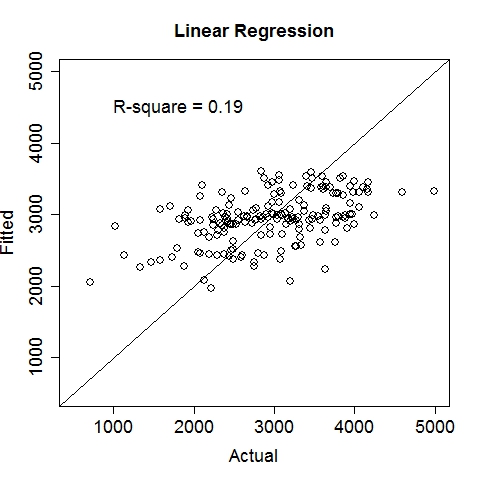
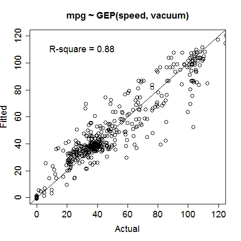
Gas MileageData were collected on Oct 1st, 2015, using an ODBII bluetooth sensor and an Android tablet running the "Torque" application. Variable: MPG (Miles per gallon, target variable), Speed (Meters/second), TurboBoostVacuumGauge (psi). Dataset is contributed by zekemo on statcrunch.com Data file: MPGdata.txt 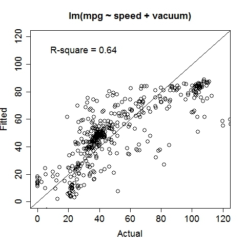
Building Energy EfficiencyThis study assesses the heating load and cooling load requirements of buildings (that is, energy efficiency) as a function of building parameters. Data source: UCI Machine Learning Repository Variables: Heating_Load (target), Relative_Compactness, Surface_Area, Wall_Area, Roof_Area, Overall_Height, Orientation, Glazing_Area, Glazing_Area_Distribution. The dataset (input_heating.txt) is randomly split into two parts for training (90%) and validation (10%): Training: train_heating.txt Validation: valid_heating.txt. Results of linear regression and composite regression are demonstrated below. Performance of Linear Regression: 
Performance of Composite Regression (better): 
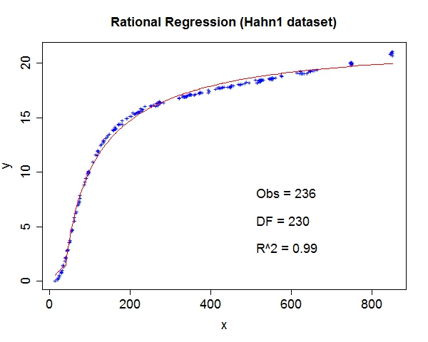
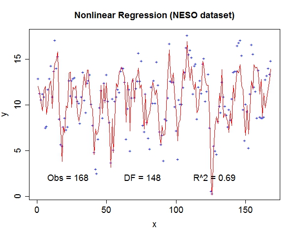
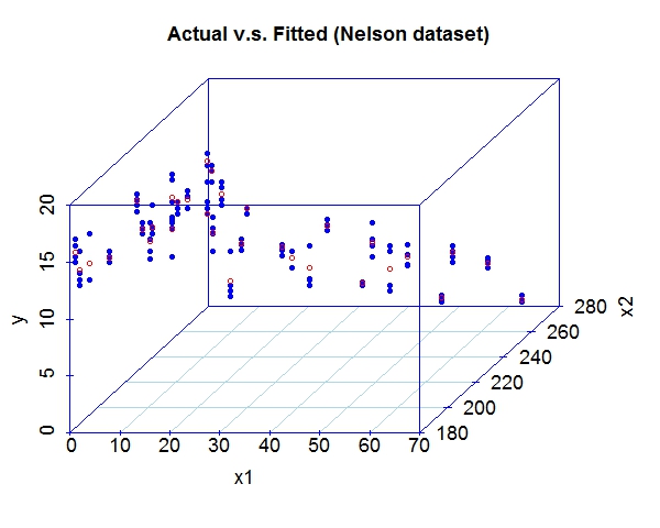
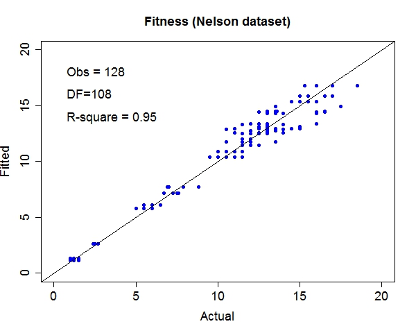
Miscellaneous TestsData source: StRD 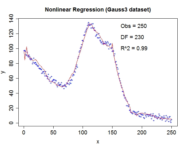

That about wraps it up. We've discussed the prospect of letting machines to learn more freely and provided a tool to explore this exciting area. For questions and discussion, welcome to contact me at yliu67 at wisc dot edu. Footnotes
|