MobLab
Guides
Aa

Consumer Choice: Cobb Douglas

Game Description

In this MobLab game, students are introduced to the Cobb-Douglas utility function. In the game, a panda must allocate a sum of money between two types of sushi with given prices. A player knows the utility from the next piece of each type and chooses one piece at at time until the budget is depleted.

Learning Objective 1: Marginal Utility Per Dollar

When allocating a fixed budget, sequentially choosing the item offering the highest marginal utility per dollar will generally lead to the utility-maximizing budget allocation.

Learning Objective 2: Familiarity with Cobb Douglas Utility

Students will gain familiarity with some of the implications of the Cobb Douglas utility function, including the result that an item’s optimal budget share is equal to the ratio of its exponent to the sum of all exponents.

Learning Objective 3: Monotonic Transformations

A monotonic transformation of a utility function (e.g., multiplying by two) does not affect the utility-maximizing consumption bundle.

Brief Instructions

The game proceeds in rounds, with one decision problem per round. We created 8 problems, from which you can choose any subset. Use the Add Round to add a problem, and the X to remove it from the list.

The analytical solution for each problem yields integer quantities. The player choosing the piece offering higher utility per dollar will find the optimum.

Note: To ensure marginal utilities are well defined, we start each problem with the player having chosen one of each piece. The problems fit together to highlight various features of utility in general and the Cobb Douglas utility function in particular.

Problem 1

u(x,y)=40x0.5y0.5, with Px=$1, Py=$1 and Budget=$12, yielding x*=6 and y*=6. Equal exponents summing to 1 with equal prices makes this a straightforward first problem since students spend 0.5/(0.5+0.5)=50% of their allocated budget on both x and y.

Problem 2

u(x,y)=40x0.5y0.5, with Px=$2, Py=$1 and Budget=$12, yielding x*=3 and y*=6. We take problem 1 and double the price of x. As the player still optimally spends half of her budget on each good, she purchases half as much x.

Problem 3

u(x,y)=40x0.5y0.5, with Px=$4, Py=$2 and Budget=$24, yielding x*=3 and y*=6. Taking problem 2 and doubling both prices and the budget does not change the utility-maximizing quantities.

Problem 4

u(x,y)=40x0.25y0.75, with Px=$1, Py=$1 and Budget=$8, yielding x*=2 and y*=6. Unequal exponents make this slightly more challenging, although prices are equal and the exponents still sum to one.

Problem 5

u(x,y)=80x0.25y0.75, with Px=$1, Py=$1 and Budget=$8, yielding x*=2 and y*=6. Taking problem 4 and doubling all utility values (by doubling the coefficient) does not affect the optimal budget allocation.

Problem 6

u(x,y)=200x0.2y0.8, with Px=$1, Py=$2 and Budget=$20, yielding x*=4 and y*=8. This problem forms the basis for a second set of problems with unequal exponents AND unequal prices. Exponents summing to one make it easy to see that the student optimally spends 20% on x and 80% on y.

Problem 7

u(x,y)=200x0.1y0.4, with Px=$1, Py=$2 and Budget=$20, yielding x*=4 and y*=8. Taking problem 6 and halving both exponents does not change the utility-maximizing allocation. The optimal allocation still entails spending 0.1/(0.1+0.4)=20% on x.

Problem 8

u(x,y)=200x0.3y1.2, with Px=$1, Py=$2 and Budget=$20, yielding x*=4 and y*=8. Taking problem 7 and tripling both exponents does not change the utility-maximizing allocation because the ratio of an exponent to the sum of exponents does not change.

Results

The end of game results highlight the optimal allocation of each type of sushi and how frequently your students followed the optimal decision rule.

Figure 1: Outcome Across Problems

First, we present a table (Figure 1) which displays the percentage of students who maximized their utility (indicated here by the column % Answering Correctly).

Figure 2: Per-Problem Details Table
Figure 3: Distribution of Purchases

In the "Per-problem Details" section we show a summary table of each problem (Figure 2) and their optimal allocation of goods based on budget constraints. We then present a chart (Figure 3), showing how purchases of Good X are distributed in each problem. Click the radio buttons to toggle which problem is shown in the distribution chart.
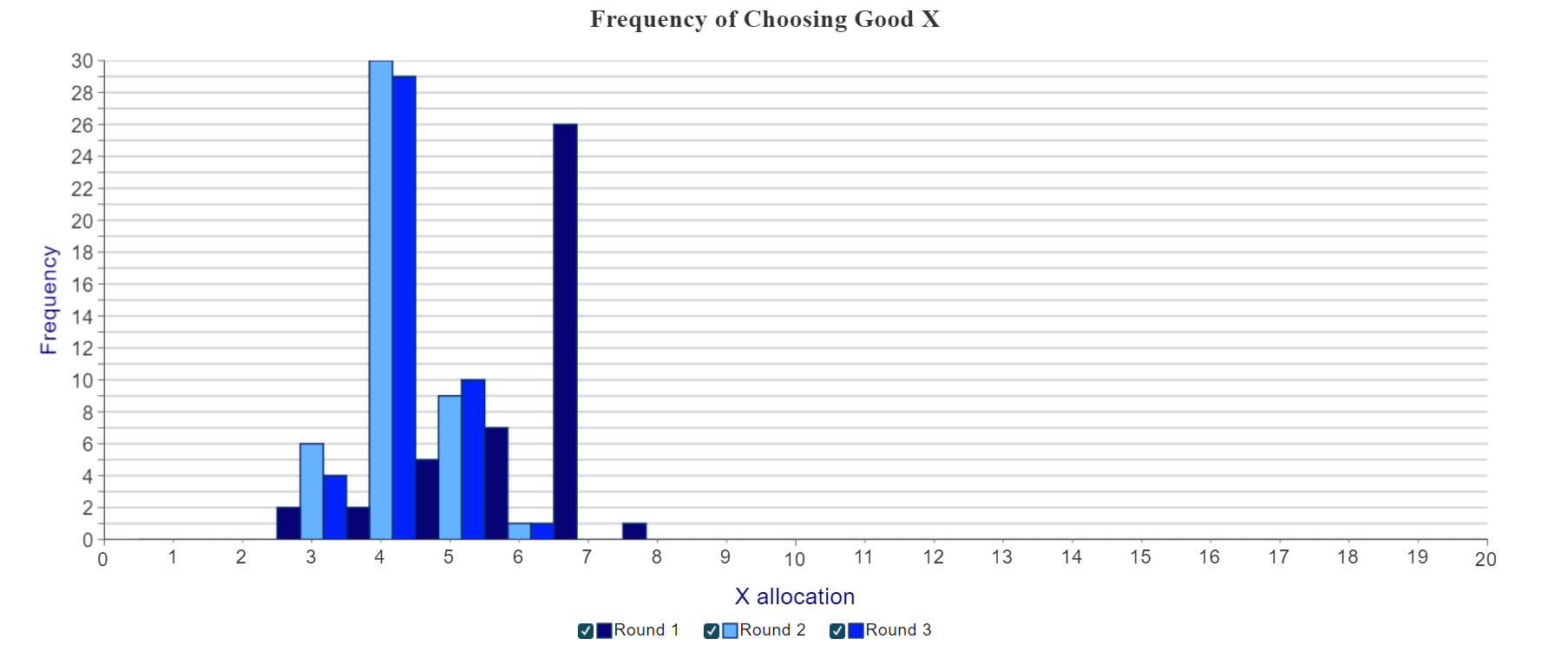
Figure 4: Frequency of Choices

Next, we present a graph showing the frequency of choices of Good X across all rounds played (Figure 4).

Note that you can choose which round(s) to include in the graph. Simply click on the checkbox next to each item in the legend.
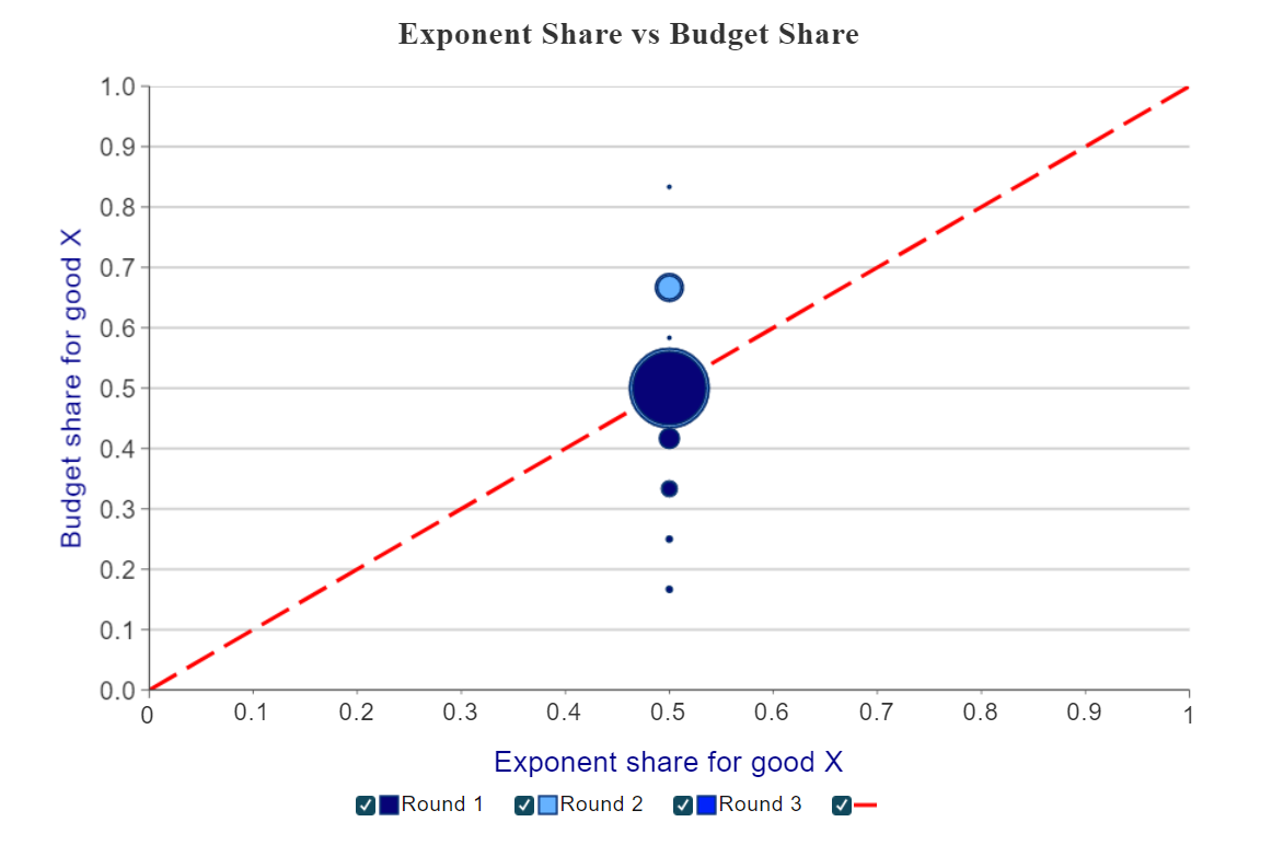
Figure 5: Exponent vs. Budget Share

Finally, we present a graph (Figure 5) showing the relationship between the exponent and budget share for Good X across rounds. A shaded circle is displayed for each round, with larger circles indicating a greater number of observations. When a student is maximizing her utility, her budget share of Good X will be equal to her exponent share of Good X (shown by the dashed red line).

Note: Because this is a single player game, there are no robot strategies.

tiled icons