Results
For most of the primary teaching goals, you will want to show convergence to the equilibrium prediction. We suggest focusing on price convergence, as it is not uncommon to have a one or two "missing" transactions. Price convergence is most clearly demonstrated by comparing transaction prices in early periods with those in later periods.

Use the Go To menu (Figure 1) to view a different period of a multi-period game or to view a different game if you have used one of the Replay options.
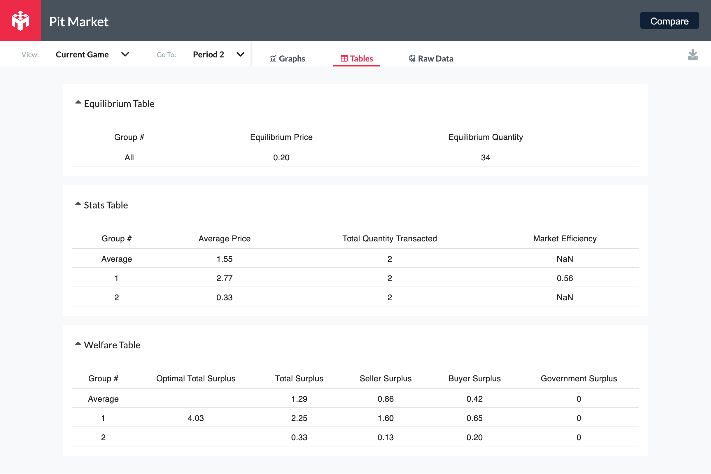
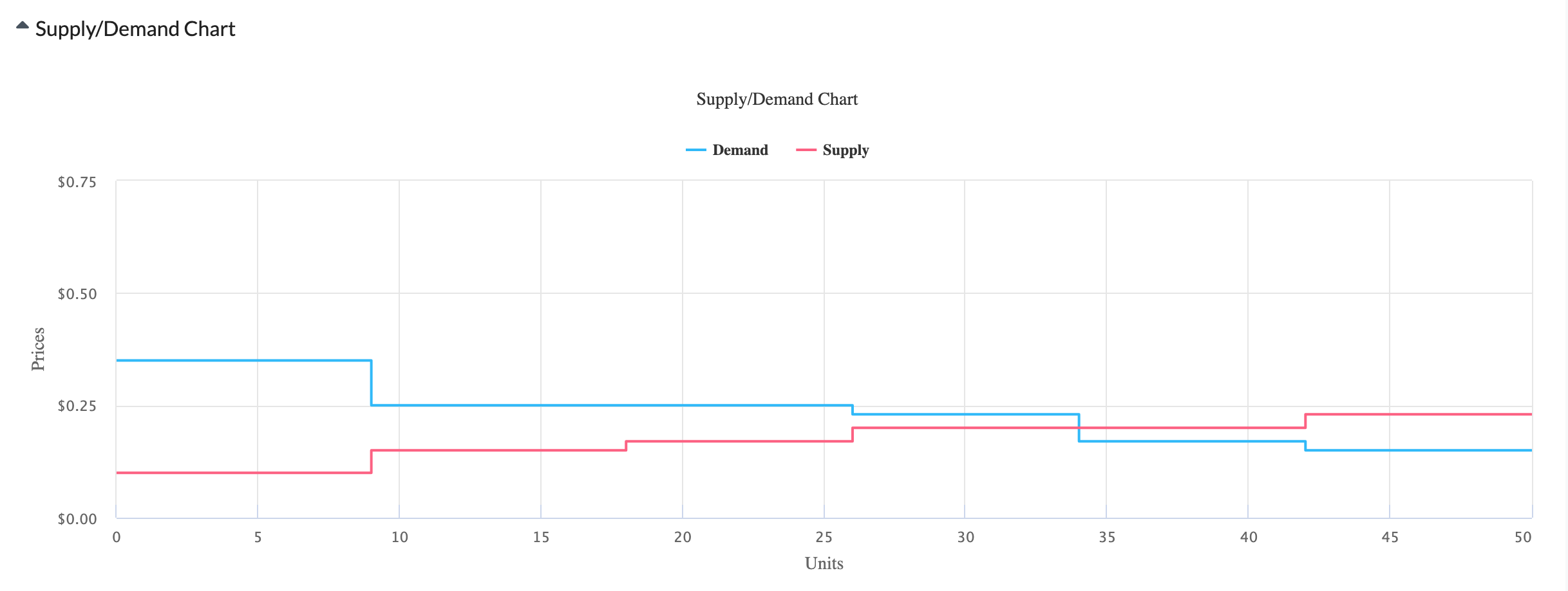
The Results display is divided into three tabs: the Graphs, Tables, and Raw Data. Tables (Figure 2) contains key statistics about each group's performance and decision making, while Graphs (Figure 3 and Figure 4) contains graphs depicting each group's market activities.

Click on the Tables option in the results screen to reveal the summary table of outcomes (Figure 2). The table allows comparison between the equilibrium market outcome and group outcomes for each round of play. We present average price, the number of transactions, consumer and producer surplus, and government surplus for the market.
There are two tables assessing group level and average performance (across groups) in a trading period. The first table presents average price, total quantity transacted, and market efficiency (Figure 4). Market Efficiency is the ratio of realized surplus to maximal surplus available. The average statistics are useful for comparisons across rounds or to compare a market without intervention to a market with intervention.

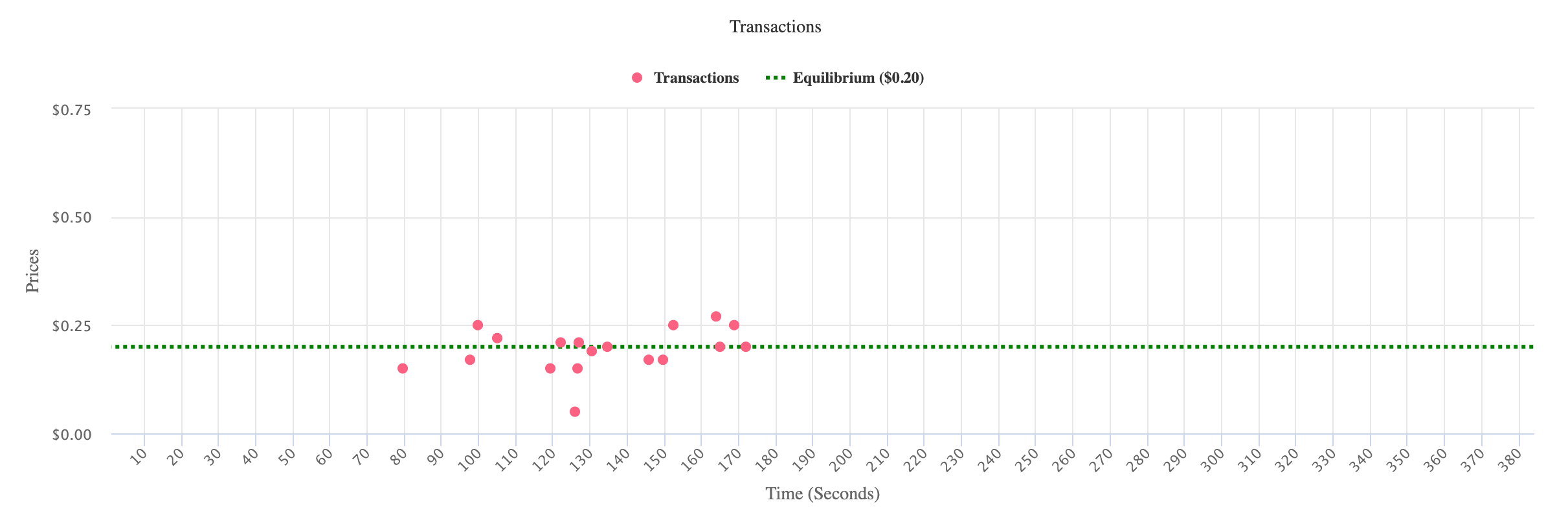
Click on the Graphs tab in the results screen to reveal the supply and demand graph and the transactions graph for the market. In each period, there are two charts for each group: on the top, the supply and demand chart (Figure 3) resulting from student costs and valuations; and the Transaction Chart on the bottom (Figure 4). With price on the vertical axis and time on the horizontal, every transaction is plotted. With repetition, transaction prices will cluster around the equilibrium price depicted in the graph.
In addition to looking at price convergence, you could also compare early periods and later periods in terms of quantities transacted and resulting market surplus.
Note that especially with shorter round durations, it is not uncommon that the quantity transacted is smaller than predicted even if price qualitatively converges to the equilibrium price. This will affect realized surplus.

Within the Graphs tab in the results screen, the transactions and equilibrium price in the selected round can also be viewed (Figure 4). Individual transactions are plotted with price on the vertical axis and time on the horizontal.* With repetition, transaction prices will cluster around the equilibrium price depicted in the graph. In addition to looking at price convergence, you could also compare early periods and later periods in terms of quantities transacted and resulting market surplus.
NOTE 1: *The Supply and Demand and Transactions graphs are plotted according to the same y-axis limit (~130% of the max value/cost configured). Transactions with prices greater than the y-axis limit will not be shown!
NOTE 2: Especially with shorter round durations, it is not uncommon that the quantity transacted is smaller than predicted even if price qualitatively converges to the equilibrium price. This will affect realized surplus.
