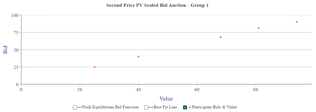
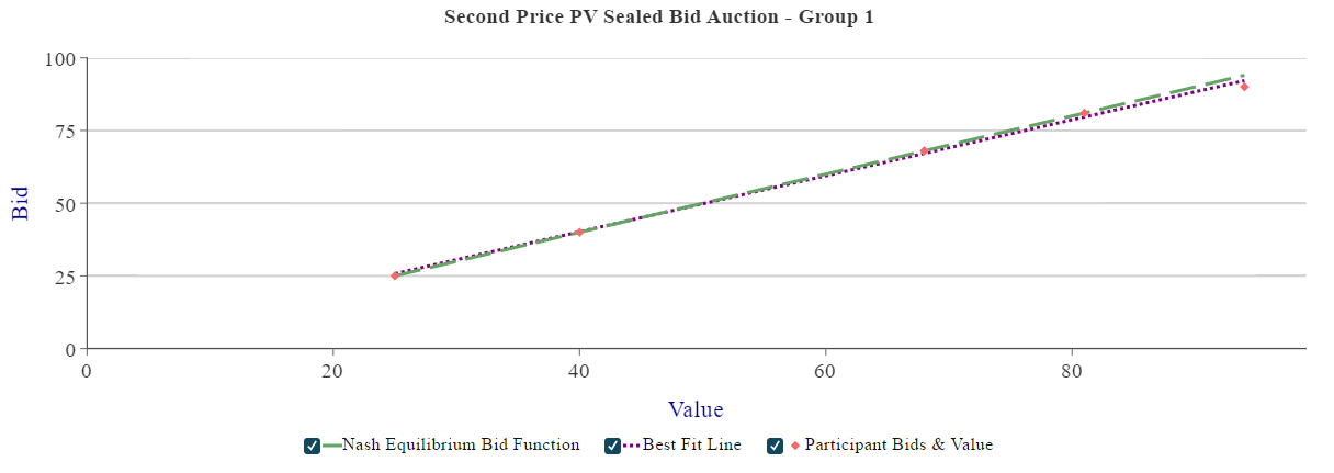
Describe the private value auction setting as a game with the set of bidders \(N = \{1,2,\cdots,n\}\). For each bidder \(i\), he/she obtains value \(v_i\), which is randomly drawn from a uniformly distributed interval \(v_i \in [\underline{v}, \bar v]\) according to the cumulative distribution function \(F_i(.)\), where \(\underline v\) is the lowest bidder value and \(\bar v\) is the highest bidder value from the configuration setting. We assume that the draw of \(v_i\) is independent across \(i\).
We assume that the distribution function is common knowledge and the true value of \(v_i\) is only known to bidder \(i\). Also, we use the \(n-1\) cumulative distribution functions \(F_j(.)\), \(j\neq i\), to form beliefs about the type \(v_{-i}\) of the other bidders. The payoff of a player who does not get the good is normalized to zero, and the payoff of a bidder who gets the good and pays a price \(p \geq 0\) is \(u_i= v_i-p\).
First Price
To complete the derivation of equilibrium bidding strategy of a sealed-bid first-price auction, we shall assume that bidder \(i\)'s equilibrium bid is increasing in his/her own valuation. That is, if \(v_i' > v_i''\), then \(s_i(v_i') > s_i(v_i'')\). It ensures that each bidder's bid function is invertible, which means that bidder \(i\)'s type is given by the inverse function of the bidder's strategy, \(s_i^{-1}(b)\). The probability of \(i\)'s bid is higher than \(j\)'s bid is thus
\(\Pr(b_i > s_i(v_i)) = \Pr(s_j^{-1}(b_i)>v_j)=F_j(s_j^{-1}(b_i)).\)
Based on independent types distribution, the expect payoff of bidder \(i\) in a first-price sealed-bid auction is
\(E_{v_{-i}}[u_i(b_i,s_{-i}(v_{-i});v_i|v_i)] = \Pi_{j\neq i}[F_j(s_j^{-1}(b_i))]\times(v_i-b_i)\).
Under the game setting, bidder \(i\)'s beliefs on others' types is the same, \(\forall i\). The maximization problem is
\(\max_{b\geq 0} E_{v_{-i}}[u_i(b_i,s_{-i}(v_{-i});v_i|v_i)] = [F(s^{*-1}(b))]^{n-1}\times(v_i-b_i)\).
Assuming an interior solution we can write down the first-order condition as follows
\(-[F(s^{*-1}(b))]^{n-1}+(n-1)[F(s^{*-1}(b))]^{n-2}f(s^{*-1}(b))\frac{ds^{*-1}(b)}{db}(v_i-b)=0\).
In order that the profile of bidding strategies \((s_1(.),\cdots,s_n(.)) = (s^*(.),\cdots,s^*(.))\) be a Bayesian Nash Equilibrium, \(b = s^*(v)\) has to be a solution to the above first order condition. Moreover, with \(\frac{ds^{*-1}(b)}{db} = \frac{1}{s^{*'}(s^{-1}(b))}\), the first order condition can be rewritten as
\(-[F(v)]^{n-1}+\frac{(n-1)[F(v)]^{n-2}f(v)(v-b)}{s^{*'}(v)}=0\).
Rewriting the above equation into a differential equation, the symmetric Bayesian Nash Equilibrium Bid Function is
\(s^*(v) = v - \frac{\int_{\underline v}^v[F(x)]^{n-1}dx}{[F(v)]^{n-1}}\).
In our game setting, bidder \(i\) is randomly drawn for a uniform distribution. The equilibrium bidding strategy is therefore
\(S^*(v) = v - \frac{\int^v_0 x^{n-1}dx}{v^{n-1}} = (\frac{n-1}{n})v\).
Second Price
The payoff function of each bidder \(i\) is
\(u_i(b_i,b_{-i};v_i) = \begin{cases} v_i - b_i^*, &\text{ if } b_i>b_j, \forall j \neq i, \text{ and } b_i \equiv \max_{j\neq i }\{b_j\}; \\0, &\text{ if } b_i \leq b_j, \text{for some } j\neq i. \end{cases}\)
Given that a bidder's action is his/her bid, a bidder's strategy assigns a bid to each of the bidder's types. The strategy for a player \(i\) is a function \(s_i:[\underline v,\bar v]\rightarrow \mathbb{R}_+\) that assigns a nonnegative bid to each of his/her possible valuations.
The expected payoff of bidder \(i\) with private valuation \(v_i\), given strategies used by the other bidders \(s_j(.),\ j\neq i\), is
\(E_{v_{-i}}[u_i(b_i,s_{-i}(v_{-i});v_i|v_i)] = \Pr(i \text{ wins and pays } b_i )\times(v_i-b_i)+\Pr(i \text{ loses })\times 0\).
Consider the cases of a bidder who is bidding below his valuation, \(b_i < v_i\). There are three possible cases with respect to the other \(n-1\) bids:
- Case 1
Bidder \(i\) is the highest bidder, in which case \(i\) wins and pays a price \(p < b_i\). Instead of bidding \(b_i\), player \(i\) would have bid \(v_i\), then he/she would still win and pay the same price, so in this case bidding his/her valuation is indifferent to bidding \(b_i\).
- Case 2
The highest bidder \(j\) bids \(b_j^{*}>v_i\), in which case \(i\) loses. Instead of bidding \(b_i\) bidder \(i\) would have bid \(v_i\) then he/she would still lose to \(b^*_j\), so in this case bidding his/her valuation is indifferent to bidding \(b_i\)
- Case 3
The highest bidder \(j\) bids \(b_j^*\) with \(b_i < b_j^*< v_i\), so that \(i\) does not win. If instead bidder \(i\) would have bid \(v_i\), he/she would have won the auction and received a payoff of \(u_i=v_i-b_j^*>0\), making this a profitable deviation, so in this case bidding his/her valuation is strictly better than bidding \(b_i\).
We can also show that bidding bidder \(i\)'s own valuation is also weakly dominant bidding \(b_i >v_i\). The fact that every player has a weakly dominant strategy, \(s_i(v_i) = v_i\), implies that each player bidding his valuation is a Bayesian Nash Equilibrium in weakly dominant strategies.1


